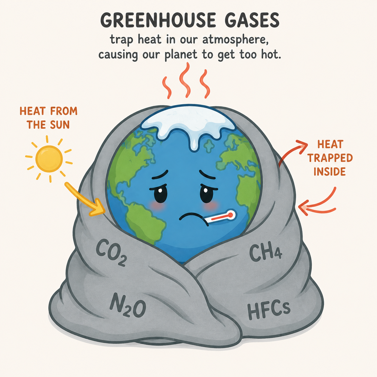
Climate Change Jerk-Continuous Growth-Constant Framework
The fundamental concern is no longer just how fast the climate is changing. It is how rapidly the rate of change itself is changing.This is a significant escalation in the level of concern. We are no longer examining simply exponential warming. We are investigating a climate system in which the rate of acceleration is itself changing, potentially amplifying an already alarming trajectory.
Daniel Brouse¹, Sidd Mukherjee²
¹ Climatologist, Economist
² Physicist
November 20, 2026
Adaptive Nonlinear Climate Acceleration Model
The updated framework extends the original nonlinear acceleration model by incorporating the third derivative of the climate system’s changing energy state. It accounts for the fact that feedback amplification does not simply increase the rate of warming or its acceleration; it also changes how rapidly that acceleration develops.
The central mathematical development is to make the growth constant time-dependent and allow its rate of change, acceleration, and jerk to evolve continuously in response to observed climate-system behavior.
Simplified Overview
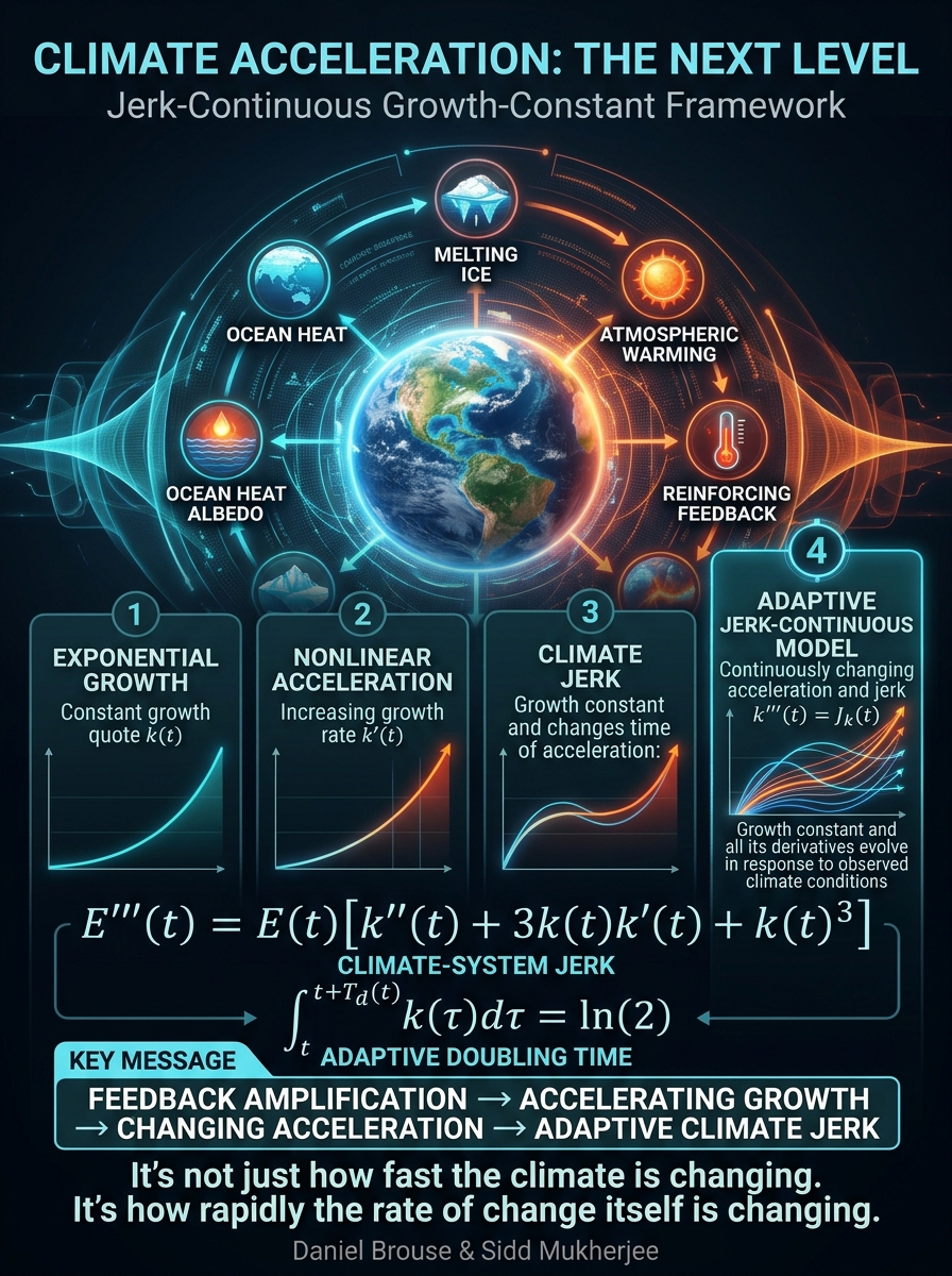
CLIMATE SCIENCE: WE’VE MOVED BEYOND SECOND-DERIVATIVE ANALYSIS.
Our climate model has evolved.
In 2025, we recognized that the scale of observed acceleration demanded a more advanced mathematical framework. Now, we’re taking the next step: an adaptive, jerk-continuous growth-constant model.
What does that mean?
We’re no longer examining just how fast the climate is warming, or how rapidly warming is accelerating. We’re examining how rapidly that acceleration itself is changing as interacting climate feedbacks amplify Earth’s energy imbalance.
The new framework incorporates:
- A continuously evolving growth constant.
- Changing rates of acceleration.
- Third-derivative climate-system behavior (jerk).
- Adaptive feedback amplification.
- Time-dependent doubling intervals.
Most importantly, the model does not assume that climate jerk remains constant. It estimates changing growth behavior from observations, allowing the framework to adapt as the climate system evolves.
This represents a significant progression beyond conventional exponential-growth models.
It’s not just how fast the climate is changing. It’s how rapidly the rate of change itself is changing.
Our updated mathematical framework:
Jerk-Continuous Growth-Constant Framework
By Daniel Brouse and Sidd Mukherjee.
Read the research and analysis:
1. Original Nonlinear Acceleration Framework
The starting point remains the discrete doubling-time formula:
Td = ln(2) / ln(1 + r)
Where:
Td = doubling time
r = fractional growth rate
ln = natural logarithm
For continuous exponential growth:
Td(t) = ln(2) / k(t)
Where k(t) represents the time-dependent growth constant.
As feedback amplification increases k(t), doubling times contract.
2. Adaptive Jerk-Continuous Growth-Constant Model
We define the climate-system energy state as E(t), representing the evolving excess-energy imbalance or another consistently defined climate-system indicator.
The governing equation becomes:
dE/dt = k(t)E(t)
Unlike the original exponential model, the growth constant is no longer assumed to be fixed or predetermined. It evolves continuously in response to changing climate-system conditions and feedback amplification.
Its evolution is described through successive derivatives:
k'(t) = dk/dt
k”(t) = d²k/dt²
k”'(t) = d³k/dt³
Where:
k(t) = time-dependent growth constant
k'(t) = rate of change of the growth constant
k”(t) = acceleration of the growth constant
k”'(t) = jerk of the growth constant
Rather than assuming that these derivatives remain constant, the adaptive framework estimates their changing values from observational data.
This distinction is fundamental: the model does not impose a predetermined acceleration or jerk trajectory. It allows the growth constant and its derivatives to respond to evolving feedback conditions.
3. Adaptive Growth-Constant Formulation
The general growth-constant model is expressed as:
k(t) = k₀ + ∫₀ᵗ k'(τ)dτ
The first derivative evolves according to:
k'(t) = k’₀ + ∫₀ᵗ k”(τ)dτ
The second derivative evolves according to:
k”(t) = k”₀ + ∫₀ᵗ k”'(τ)dτ
The third derivative is allowed to vary continuously:
k”'(t) = Jₖ(t)
Where Jₖ(t) represents the time-dependent jerk of the growth constant.
This creates an adaptive, observation-driven mathematical structure in which the growth constant, its rate of change, its acceleration, and its jerk are not restricted to fixed coefficients.
For an initial approximation, a cubic representation remains useful:
k(t) = k₀ + αt + (β/2)t² + (γ/6)t³
However, this is a simplified approximation in which the third derivative is constant:
k”'(t) = γ
The more advanced model replaces the constant γ with a time-dependent function:
k”'(t) = Jₖ(t)
Consequently, the cubic approximation becomes a continuously adaptive model capable of representing changing feedback amplification rather than imposing a fixed growth trajectory.
4. The Third Derivative: Climate-System Jerk
Starting with the governing energy-growth equation:
E'(t) = k(t)E(t)
The second derivative becomes:
E”(t) = E(t)[k'(t) + k(t)²]
The third derivative becomes:
E”'(t) = E(t)[k”(t) + 3k(t)k'(t) + k(t)³]
This is the climate-system jerk equation.
We define:
Jₑ(t) = E”'(t)
It captures three interacting components:
- Growth-constant curvature: k”(t)
- Growth-feedback coupling: 3k(t)k'(t)
- Nonlinear exponential amplification: k(t)³
Together, these terms describe how the climate system’s energy-growth acceleration changes over time.
Importantly, climate-system jerk Jₑ(t) and growth-constant jerk Jₖ(t) are distinct mathematical quantities. The former measures the third derivative of the energy state; the latter measures the third derivative of the growth constant.
The adaptive framework incorporates both.
5. Updated Doubling-Time Equation
The original continuous doubling-time equation assumes a constant growth rate over the doubling interval.
With a continuously changing growth constant, the mathematically exact formulation becomes:
∫ₜᵗ⁺ᵀᵈ⁽ᵗ⁾ k(τ)dτ = ln(2)
This equation determines doubling time from the accumulated growth rate over the entire interval.
For the simplified cubic approximation:
k₀Td + (α/2)Td² + (β/6)Td³ + (γ/24)Td⁴ = ln(2)
For the fully adaptive model, the integral formulation remains the governing equation:
∫ₜᵗ⁺ᵀᵈ⁽ᵗ⁾ k(τ)dτ = ln(2)
The instantaneous approximation remains:
Td(t) ≈ ln(2) / k(t)
As feedback amplification increases the growth constant, the exact doubling interval contracts.
6. Complete Adaptive Framework
JERK-CONTINUOUS GROWTH-CONSTANT FRAMEWORK
Governing energy-growth equation:
E'(t) = k(t)E(t)
Adaptive growth constant:
k(t) = k₀ + ∫₀ᵗ k'(τ)dτ
Changing growth-constant acceleration:
k”(t) = k”₀ + ∫₀ᵗ Jₖ(τ)dτ
Time-dependent growth-constant jerk:
Jₖ(t) = k”'(t)
Climate-system acceleration:
E”(t) = E(t)[k'(t) + k(t)²]
Climate-system jerk:
Jₑ(t) = E”'(t)
Jₑ(t) = E(t)[k”(t) + 3k(t)k'(t) + k(t)³]
Exact time-dependent doubling:
∫ₜᵗ⁺ᵀᵈ⁽ᵗ⁾ k(τ)dτ = ln(2)
7. Observation-Driven Model Implementation
The advanced framework estimates the growth constant and its derivatives from observed climate-system behavior rather than imposing fixed mathematical coefficients.
The implementation follows four principal steps:
- Estimate k(t) from the observed evolution of the selected climate-system energy indicator.
- Calculate k'(t) to measure changes in the growth constant.
- Calculate k”(t) to measure acceleration in the growth constant.
- Estimate k”'(t) as a time-dependent quantity to capture changing jerk and feedback amplification.
The resulting model continuously updates its representation of the climate system as new observations become available.
Because higher-order derivatives amplify observational noise, the implementation must account for measurement uncertainty, temporal resolution, smoothing sensitivity, and the distinction between persistent trends and internal climate variability.
The model should also test whether the observed higher-order behavior is statistically distinguishable from alternative growth models.
8. Scientific Interpretation
The progression of the framework is:
First derivative (E’): Growth velocity.
Second derivative (E”): Growth acceleration.
Third derivative (E”’): Rate of change of acceleration.
Adaptive growth constant (k(t)): Continuously evolving growth behavior.
Adaptive growth-constant derivatives (k’, k”, k”’): Changing growth velocity, acceleration, and jerk.
The distinction is important.
A conventional exponential-growth model assumes a constant growth rate. A nonlinear acceleration model allows that rate to increase. The jerk-continuous framework goes further by examining how the acceleration itself changes as feedback processes interact.
The advanced adaptive model goes one step further: it does not assume that climate jerk remains constant. It estimates the changing behavior of the growth constant and its derivatives from observations, allowing the mathematical framework to evolve alongside the climate system.
9. Updated Authorship Statement
Daniel Brouse and Sidd Mukherjee
Our climate model has evolved from nonlinear acceleration analysis into an adaptive, jerk-continuous growth-constant framework.
We are no longer examining only how rapidly the climate system is warming, or even how rapidly that warming is accelerating. We are examining how rapidly the acceleration itself is changing as interacting feedback mechanisms amplify the system’s energy redistribution.
The critical mathematical development is the introduction of a continuously evolving growth constant whose derivatives capture changing feedback amplification, coupled with a third-derivative measure of climate-system behavior.
Unlike conventional exponential models or simplified cubic approximations, the advanced framework does not impose a fixed growth trajectory or assume constant climate jerk. It allows the growth constant, its acceleration, and its jerk to evolve in response to observed climate-system behavior.
This moves the analysis beyond conventional exponential warming models toward an adaptive framework for investigating higher-order nonlinear acceleration, feedback coupling, and increasingly compressed doubling times.
The fundamental concern is no longer just how fast the climate is changing. It is how rapidly the rate of change itself is changing.
Singularity
As individual feedbacks emerge, couple, and organize into self-reinforcing feedback networks, these networks will increasingly interact and converge into a unified, interconnected system approaching climate-system singularity.
Feedback Loops → Tipping Points → Feedback Loop and Tipping-Point Network → Acceleration → Domino Effect
Feedback loops amplify climate change and can push interconnected Earth systems past critical tipping points. As tipping points are crossed, they can trigger additional feedback loops and destabilize other climate systems. This cascading "Domino Effect" compresses timescales, accelerates change, and increases the risk of rapid, nonlinear climate transformations.
Current Status: Climate Tipping Point Crisis
Easy-to-Read Resources