Start with: Framework for Nonlinear Climate Outcomes (Public Access Version)

Probability Distribution (Model Scenario)

A Theoretical Model of Coupled Feedback Amplification, System-State Transitions, and Future Climate Trajectories

A Theoretical Model of Coupled Feedback Amplification, System-State Transitions, and Future Climate Trajectories

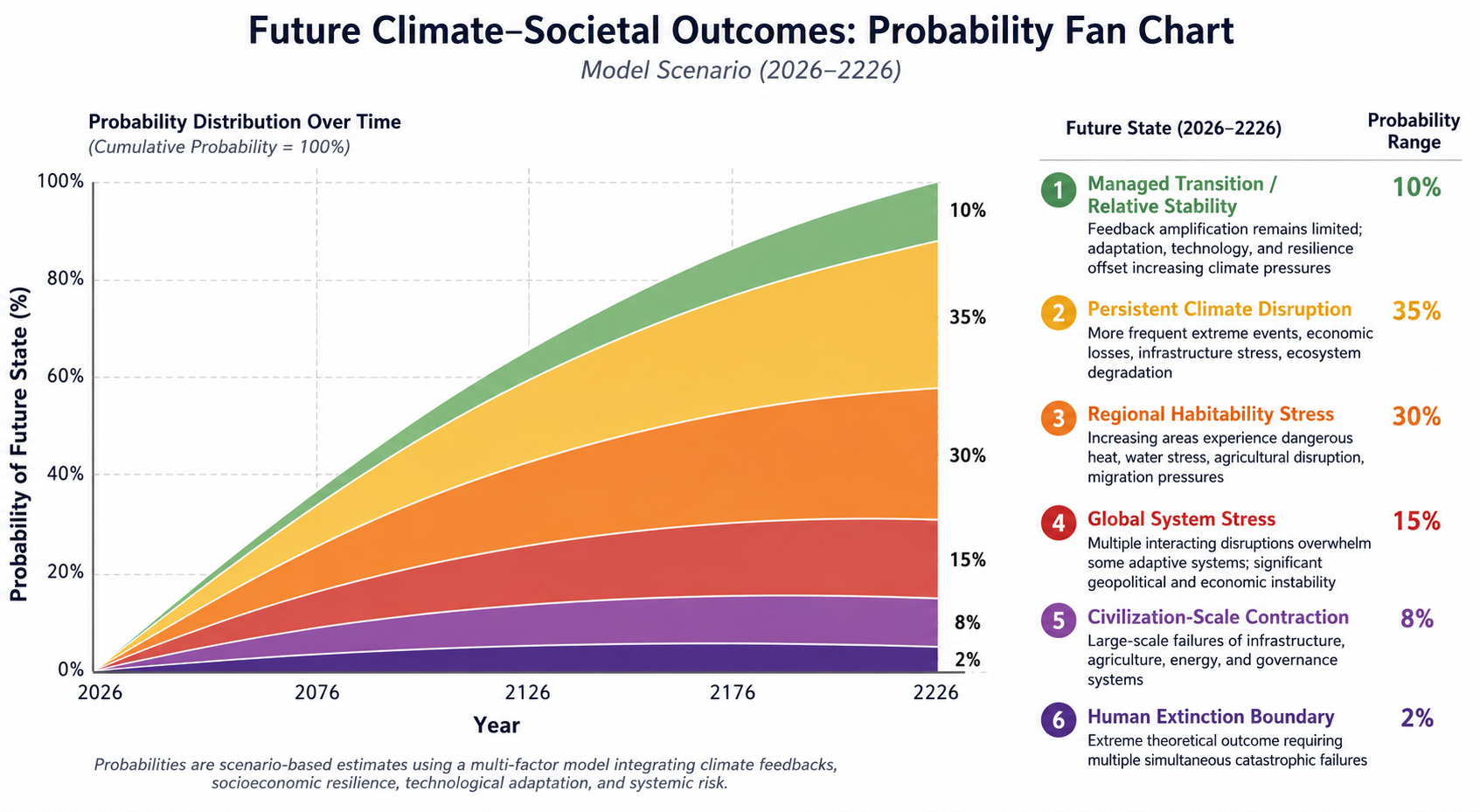
The distribution is not intended to be a literal prediction of where humanity will be in exactly 200 years. A 200-year horizon necessarily involves enormous uncertainty—seven generations means changes in technology, governance, economics, and adaptation capacity that cannot be known today.

The main purpose of the graph is to emphasize that human extinction remains a very low-probability outcome across the modeled scenarios. The more likely risks involve increasing climate disruption, ecosystem stress, and challenges to human systems.

Given that distinction, the most important actions are clear: reduce the primary driver of warming by transitioning away from fossil fuel combustion while simultaneously accelerating adaptation and resilience efforts. The goal is not to focus on an unlikely worst-case outcome, but to reduce the probability of disruptive pathways and improve the chances of a stable, adaptable future.

Abstract

Climate change is often represented as a sequence of approximately linear responses to increasing radiative forcing. However, complex Earth systems do not evolve as isolated variables responding independently to external perturbations. They behave as interconnected nonlinear systems in which feedback interactions can amplify, redistribute, and accelerate responses over time.

This paper presents a theoretical framework—the Nonlinear Acceleration Framework (NAF)—for describing climate evolution as a coupled dynamical system governed by interacting physical, ecological, and societal processes. The framework proposes that climate impacts should not be evaluated solely through individual trends but through the changing acceleration of interconnected system variables.

The central hypothesis is that the Earth system can experience emergent nonlinear acceleration when multiple feedback mechanisms become coupled. In this formulation, relatively small perturbations may propagate through interconnected subsystems, creating cascading responses analogous to network failures in other complex systems.

The paper introduces a conceptual probability envelope rather than a deterministic prediction. The envelope represents a range of possible future trajectories, extending from relative climate stabilization through increasing disruption, regional habitability loss, civilization-scale stress, and theoretical upper-bound outcomes involving human extinction. These pathways are constrained by fundamental physical principles, including conservation of energy, radiative transfer, thermodynamics, ocean heat capacity, atmospheric moisture relationships, and nonlinear dynamical behavior.

The framework does not claim that extreme outcomes are inevitable. Rather, it proposes that increasing coupling among climate subsystems may shift probability distributions away from stable states and toward progressively more disruptive states.

This theoretical model provides a foundation for future mathematical development through stochastic dynamical systems, Bayesian inference, and computational simulations.

Keywords

Nonlinear climate dynamics; climate feedbacks; complex systems; chaos theory; tipping cascades; Earth system science; probability envelope; nonlinear acceleration; coupled systems; state-space modeling

1. Introduction

The Earth’s climate system is not a collection of independent components. It is a coupled network consisting of interacting physical, chemical, biological, and human systems. The atmosphere, oceans, cryosphere, biosphere, and human infrastructure exchange energy and information continuously.

Traditional approaches often analyze climate impacts through individual variables:

• atmospheric temperature,
• ocean heat content,
• sea-level rise,
• precipitation patterns,
• ecosystem responses.

While these measurements remain essential, a complex systems perspective suggests that the behavior of the whole system cannot always be inferred from isolated components.

A defining characteristic of complex nonlinear systems is that the response of the system may not be proportional to the initial disturbance.

A small perturbation can:

1. activate feedback mechanisms,
2. alter system conditions,
3. increase the probability of additional responses,
4. create interactions among previously separated processes.

This behavior is commonly described as emergence.

The central premise of the Nonlinear Acceleration Framework is that climate change should be evaluated not only by the magnitude of change, but by the changing rate of change and the increasing interaction among feedback pathways.

A linear interpretation assumes:$$Change \propto Forcing$$Change∝Forcing

A nonlinear interpretation considers:$$\frac{dX}{dt}=f(X,t)$$

where the evolution of the system depends not only on external forcing but also on the internal state of the system itself.

In this formulation, the climate system can move through different dynamical regimes.

A relatively stable regime may transition into:

• increasing variability,
• amplified extremes,
• cascading feedback activation,
• regional system failures,
• broader societal disruption.

The purpose of this paper is to establish a theoretical structure for describing these transitions.

The framework is built around three concepts:

1. Nonlinear Acceleration

The rate of change of climate variables may itself change over time.

2. The Domino Effect

Individual feedback mechanisms may become connected, allowing disturbances to propagate through the Earth system.

3. Probability Envelopes

Future outcomes should be represented as distributions of possible trajectories rather than single deterministic forecasts.

2. Foundations of the Nonlinear Acceleration Framework

2.1 Climate as a Complex Adaptive System

A complex adaptive system contains:

• multiple interacting components,
• feedback loops,
• thresholds,
• nonlinear responses,
• emergent behavior.

The climate system satisfies these characteristics.

Represent the Earth system as:$$S(t)= \{A,O,C,B,H\}$$

where:

• A = atmosphere
• O = ocean system
• C = cryosphere
• B = biosphere
• H = human systems

The evolution of the system is:$$\frac{dS}{dt}=F(S,E,t)$$

where:

• F represents internal system dynamics,
• E represents external forcing.

The critical insight is that:$$F(S,t)\neq constant$$

The system itself changes as conditions evolve.

A warmer ocean is not simply the same ocean at a higher temperature. It has altered:

• circulation patterns,
• evaporation rates,
• atmospheric moisture content,
• biological conditions,
• ice interactions.

The system state modifies future evolution.

2.2 Acceleration as a Primary Variable

Most analyses focus on:$$X(t)$$

the value of a climate variable.

The Nonlinear Acceleration Framework introduces a second-order perspective:$$\frac{dX}{dt}$$

and:$$\frac{d^2X}{dt^2}$$

The first derivative represents the rate of change.

The second derivative represents acceleration.

A system undergoing acceleration behaves differently from a system experiencing constant change.

For example:

Linear:$$X(t)=X_0+kt$$

Accelerating:$$X(t)=X_0e^{kt}$$

where:

• k represents the growth constant.

The doubling time is:$$T_d=\frac{\ln(2)}{k}$$

A declining doubling time indicates increasing acceleration.

The framework proposes that coupled climate indicators can be evaluated through changing characteristic timescales.

2.3 Coupled Feedback Dynamics

A feedback loop occurs when a change in one component influences another component, which then feeds back into the original component.

A simplified example:$$Temperature \rightarrow Ice Loss \rightarrow Reduced Albedo \rightarrow Additional Heating$$

The initial disturbance becomes amplified.

The feedback gain can be represented as:$$G=\prod_i f_i$$

where each:$$f_i$$

represents the influence of an individual feedback process.

If:$$G<1$$

the disturbance tends to decay.

If:$$G>1$$

the disturbance tends to amplify.

The theoretical concern of nonlinear acceleration is not the existence of individual feedbacks, but the possibility that multiple feedbacks become increasingly coupled.

3. Physical Constraints on Climate Evolution

A theoretical framework must remain bounded by fundamental physical laws.

Nonlinear acceleration does not imply unlimited warming.

The Earth system operates within physical constraints.

3.1 Conservation of Energy

The climate system follows energy conservation:$$Energy_{in}-Energy_{out}=Energy_{stored}$$

Incoming solar radiation must balance outgoing radiation over time.

Changes in greenhouse gas concentrations alter the balance between incoming and outgoing energy.

However, the resulting temperature response remains constrained by:

• atmospheric composition,
• ocean heat storage,
• surface properties,
• feedback strength.

3.2 Radiative Equilibrium

The Earth emits infrared radiation according to temperature.

A simplified representation:$$F=\sigma T^4$$

where:

• F is emitted radiation,
• σ is the Stefan-Boltzmann constant,
• T is temperature.

Increasing atmospheric absorption changes the effective emission level and requires adjustment toward a new equilibrium.

The equilibrium response is not instantaneous because different components respond at different timescales.

3.3 Ocean Heat Capacity

The oceans represent a massive thermal reservoir.

The temperature response can be represented as:$$Q=mc\Delta T$$

where:

• m is mass,
• c is heat capacity,
• ΔT is temperature change.

Because oceans store enormous quantities of heat, they moderate short-term atmospheric responses.

However, stored heat also represents delayed energy release into the climate system.

3.4 Atmospheric Moisture Amplification

Atmospheric water vapor is a major climate feedback because warmer air can contain more moisture.

The relationship is nonlinear and follows thermodynamic constraints.

A warmer atmosphere increases:

• moisture capacity,
• latent heat transport,
• potential precipitation intensity.

This creates additional coupling between:

temperature,

humidity,

storms,

flooding,

and atmospheric circulation.

3.5 Physical Limits and Upper Boundaries

A critical distinction must be made between:

Earth-system destabilization

and

planetary runaway warming.

A nonlinear climate trajectory does not imply conditions comparable to Venus.

The theoretical upper boundary considered here is therefore not unlimited temperature increase, but progressive degradation of conditions required for complex human civilization.

The relevant question becomes:

Not:

“Can Earth become Venus?”

but:

“What range of Earth conditions remains compatible with current human systems?”

4. The Domino Effect:

Climate Feedbacks as a Coupled Nonlinear Network

The central premise of the Nonlinear Acceleration Framework is that climate change cannot be adequately represented as a collection of independent trends. The Earth system operates as a network of interacting processes where disturbances can propagate across multiple domains.

This section introduces the Domino Effect hypothesis: the possibility that a perturbation in one subsystem can increase the probability of changes in connected subsystems, producing a cascade of reinforcing responses.

The metaphor of falling dominoes is not intended to imply a predetermined sequence. Rather, it describes a network effect in which the state change of one component modifies the conditions of neighboring components.

In mathematical terms, the climate system can be represented as a directed graph:$$G=(V,E)$$

where:

• V represents climate, ecological, and societal components,
• E represents the interactions between components.

Each node contains a state variable:$$X_i(t)$$

and each connection contains an influence coefficient:$$C_{ij}$$

where:$$C_{ij} = \frac{\partial X_i}{\partial X_j}$$

represents how changes in one system influence another.

The complete system becomes:$$\frac{dX_i}{dt} = F_i(X_1,X_2,…,X_n,t)$$

The important property of this formulation is that the behavior of one component depends on the state of the entire network.

4.1 From Individual Feedbacks to Feedback Networks

Individual feedback mechanisms are often examined separately.

Examples include:$$Ice\ Loss \rightarrow Albedo\ Reduction \rightarrow Heating$$

or:$$Warming \rightarrow More\ Atmospheric\ Moisture \rightarrow Extreme\ Precipitation$$

or:$$Ocean\ Warming \rightarrow Marine\ Heatwaves \rightarrow Ecosystem\ Stress$$

However, nonlinear behavior emerges when these pathways interact.

A simplified network:

                 Atmospheric Warming
                         |
                         |
        --------------------------------
        |               |               |
        ↓              ↓               ↓

    Ice Loss     Ocean Heating    Soil Drying
        |              |               |
        ↓              ↓               ↓

   Albedo Loss   Marine Stress   Wildfire Risk
        |              |               |
        --------------------------------
                         |
                         ↓

              Additional Atmospheric Change

The system is no longer a chain.

It becomes a feedback network.

4.2 Feedback Coupling Strength

The effect of a single feedback can be represented as:$$F_i$$

The combined effect of multiple interacting feedbacks can be represented by:$$F_{total} = \sum_iF_i+ \sum_{i,j}C_{ij}F_iF_j$$

The first term represents independent feedbacks.

The second term represents interaction effects.

The critical theoretical proposition is that:$$\sum_{i,j}C_{ij}F_iF_j$$

may become increasingly important as coupling increases.

This represents the transition from:

a system containing feedbacks

to:

a feedback-dominated system.

4.3 Cascading Transitions

Complex systems often experience transitions when internal connections exceed stabilizing forces.

Define:$$R= \frac{Amplifying\ Connections} {Stabilizing\ Connections}$$

When:$$R<1$$

the system tends toward recovery.

When:$$R\approx1$$

the system becomes highly sensitive.

When:$$R>1$$

amplifying processes dominate.

This does not mean collapse is guaranteed.

It means the probability distribution of future states shifts.

A small disturbance occurring in a weakly coupled system may disappear.

The same disturbance occurring in a highly coupled system may propagate.

4.4 Examples of Domino-Style Interactions

Cryosphere Pathway

A simplified pathway:$$Temperature Increase$$TemperatureIncrease

↓$$Ice Reduction$$IceReduction

↓$$Surface Reflectivity Change$$SurfaceReflectivityChange

↓$$Additional Energy Absorption$$AdditionalEnergyAbsorption

↓$$Further Warming$$FurtherWarming

The initial disturbance is amplified through a secondary pathway.

Ocean-Atmosphere Pathway

$$Ocean Heating$$OceanHeating

↓$$Increased Evaporation$$IncreasedEvaporation

↓$$Atmospheric Moisture Increase$$AtmosphericMoistureIncrease

↓$$Changed Precipitation Extremes$$ChangedPrecipitationExtremes

↓$$Flooding/Drought\ Variability$$Flooding/Drought Variability

↓$$Ecosystem and Infrastructure Stress$$EcosystemandInfrastructureStress

Biosphere Pathway

$$Heat Stress$$HeatStress

↓$$Vegetation Loss$$VegetationLoss

↓$$Carbon Cycle Alteration$$CarbonCycleAlteration

↓$$Reduced Natural Buffering Capacity$$ReducedNaturalBufferingCapacity

↓$$Additional Atmospheric Changes$$AdditionalAtmosphericChanges

5. State-Space Representation of Earth-System Trajectories

A major limitation of simple forecasting is that it attempts to estimate a single future value.

Complex systems do not evolve along a single predictable path.

Instead, they occupy a region of possible states.

5.1 Defining the Climate State Vector

The Earth system can be represented as:$$X(t) = \begin{bmatrix} C\\ O\\ A\\ B\\ H \end{bmatrix}$$

where:

• C = cryosphere state
• O = ocean state
• A = atmosphere state
• B = biosphere state
• H = human system state

Each component contains multiple variables.

For example:$$O= \begin{bmatrix} Heat\\ Circulation\\ Chemistry\\ Biology \end{bmatrix}$$O=​HeatCirculationChemistryBiology​​

The complete Earth system exists as a point in a multidimensional phase space.

5.2 Climate Trajectories

The evolution of the system becomes:$$X(t+1)=F(X(t),U(t),\epsilon)$$

where:

• F represents system dynamics,
• U(t) represents external forcing,
• ϵ represents stochastic variability.

The future is therefore not a single line.

It is a collection of possible trajectories:$$\{X_1(t),X_2(t),…,X_n(t)\}$$

5.3 Stability Regions

Complex systems often contain regions called attractors.

An attractor represents a range of states toward which the system tends to evolve.

A simplified representation:

          Stable Region

              ●


       Increasing Instability


              ●


       High Stress Region


              ●


       System Transformation

The theoretical question becomes:

How does increasing nonlinear coupling affect the movement of the system between regions?

5.4 Threshold Dynamics

Thresholds occur when gradual changes produce abrupt responses.

Mathematically:$$X<X_c$$​

may produce gradual change.

But:$$X>X_c$$

may produce a nonlinear transition.

The framework treats thresholds not as isolated points but as interacting boundaries.

A single threshold crossing may alter the probability of crossing other thresholds.

6. The Conceptual Probability Envelope

6.1 Purpose

The purpose of the probability envelope is not to produce a single prediction.

Instead, it describes how the distribution of possible futures may shift as nonlinear coupling changes.

The framework defines future states as:$$S= \{S_1,S_2,S_3,…,S_n\}$$

where possible states include:

• relative stability,
• increasing disruption,
• regional habitability loss,
• systemic civilization stress,
• civilization collapse,
• theoretical extinction boundary.

6.2 Probability Distribution

The probability of each state is:$$P(S_i|F)$$

where:

• $S_i$Si​ represents a future state,
• $F$F represents the combined feedback condition.

The probability distribution must satisfy:$$\sum_iP(S_i)=1$$

As nonlinear coupling increases, the distribution may shift:

Early State:

Stability
█████████

Disruption
██

Collapse
█

Extinction
.


Later State:

Stability
███

Disruption
███████

Collapse
████

Extinction
█

The framework does not state that the upper outcomes are inevitable.

It states that increasing system coupling changes the shape of the probability landscape.

6.3 Scenario Categories

The conceptual envelope contains six broad regions.

Scenario 1:

Relative Stabilization

Characteristics:

• feedback amplification remains limited,
• adaptation remains effective,
• system coupling remains manageable.

State:$$C<0.2$$

Scenario 2:

Increasing Climate Disruption

Characteristics:

• increasing extreme events,
• infrastructure stress,
• economic impacts.

State:$$0.2<C<0.4$$

Scenario 3:

Regional Habitability Stress

Characteristics:

• increasing areas experiencing dangerous conditions,
• agricultural disruption,
• migration pressures.

State:$$0.4<C<0.6$$

Scenario 4:

Global System Stress

Characteristics:

• multiple simultaneous disruptions,
• declining adaptive capacity,
• interconnected failures.

State:$$0.6<C<0.8$$

Scenario 5:

Civilization-Scale Contraction

Characteristics:

• severe loss of infrastructure reliability,
• economic fragmentation,
• reduced technological capacity.

State:$$0.8<C<0.95$$

Scenario 6:

Human Extinction Boundary

Characteristics:

• extreme theoretical conditions,
• failure of global adaptation,
• loss of environments capable of sustaining human populations.

State:$$C>0.95$$

This represents an upper-bound possibility, not a prediction.

6.4 Interpretation

The central conclusion of the probability envelope is:

The most important variable is not only the amount of climate change, but the degree of coupling among interacting systems.

A world with large individual changes but weak coupling may remain manageable.

A world with moderate changes and strong coupling may experience cascading effects.

The framework therefore shifts the question from:

“How much warming occurs?”

to:

“How does the Earth system respond as connections among components intensify?”

7. Mathematical Development of the Nonlinear Probability Model

7.1 From Conceptual Framework to Dynamical Model

The previous sections described the Earth system as a coupled nonlinear network. This section develops a mathematical structure for representing the evolution of possible future states.

The purpose of this model is not to claim a deterministic forecast. Instead, it provides a mathematical language for describing how changes in feedback strength, coupling, and system resilience could alter the distribution of possible trajectories.

The general form of a nonlinear dynamical system is:$$\frac{dX}{dt}=F(X,t)+\eta(t)$$

where:

• X is the Earth-system state vector,
• F(X,t) represents deterministic system behavior,
• η(t) represents stochastic variability.

The inclusion of $\eta(t)$η(t) recognizes that complex systems are influenced by internal variability and unpredictable perturbations.

The system therefore evolves through both:

1. deterministic physical processes,
2. probabilistic events.

7.2 The Nonlinear Acceleration State Vector

The Nonlinear Acceleration Framework proposes that important indicators should not be evaluated only by their magnitude but also by their rate of change.

Define:$$X(t)= \begin{bmatrix} O(t)\\ L(t)\\ M(t)\\ W(t)\\ E(t)\\ S(t) \end{bmatrix}$$​​

where:

• O(t) = ocean heat state,
• L(t) = cryosphere loss state,
• M(t) = marine disturbance state,
• W(t) = atmospheric moisture/extreme weather state,
• E(t) = ecosystem stability state,
• S(t) = societal resilience state.

The system acceleration becomes:$$A(t)=\frac{d^2X}{dt^2}$$

A positive acceleration indicates increasing rates of change.

A negative acceleration indicates stabilization or recovery.

7.3 Coupling Matrix

The interaction among variables is represented by a coupling matrix:$$C= \begin{bmatrix} c_{11}&c_{12}&…&c_{1n}\\ c_{21}&c_{22}&…&c_{2n}\\ …&…&…&…\\ c_{n1}&c_{n2}&…&c_{nn} \end{bmatrix}$$

where:$$c_{ij}$$

represents the influence of variable $j$j on variable $i$i.

The system evolution becomes:$$\frac{dX}{dt}=CX+F(X)+\eta$$

If coupling coefficients remain small, individual disturbances may decay.

If coupling coefficients increase, disturbances may propagate.

7.4 The Domino Amplification Factor

Define a theoretical amplification factor:$$D=\lambda_{max}(C)$$

where:$$\lambda_{max}$$

is the largest eigenvalue of the coupling matrix.

This value represents the dominant growth tendency of the network.

Interpretation:$$D<1$$

The network tends toward stability.$$D=1$$

The network is at a critical transition.$$D>1$$

Amplifying processes dominate.

This does not imply inevitable collapse. It indicates increasing sensitivity to perturbations.

7.5 Collapse Index

To translate system dynamics into a conceptual outcome space, define:$$CI(t)= \sum_i w_iX_i(t)$$

where:

• CI = Collapse Index,
• wi​ = weighting factors.

The index is normalized:$$0\leq CI\leq1$$

Possible interpretation:

These ranges are conceptual categories, not measured probabilities.

7.6 Probability Density Over Future States

Instead of assigning one future, define a probability density:$$P(X,t)$$

The evolution of this probability distribution can be represented using a stochastic equation:$$\frac{\partial P}{\partial t} = -\nabla(FP) + \frac12\nabla^2(DP)$$

This formulation describes how possible futures spread, contract, or shift over time.

The probability envelope is therefore dynamic.

It changes as:

• feedback strength changes,
• coupling changes,
• resilience changes,
• adaptation changes.

7.7 Bayesian Interpretation

The framework can also be expressed using Bayesian updating.

Initial assumptions:$$P(S_i)$$

represent prior probability distributions.

New system information:$$D$$

updates the distribution:$$P(S_i|D) = \frac{P(D|S_i)P(S_i)} {P(D)}$$

In this theoretical framework:

• observations modify the probability landscape,
• they do not determine a single outcome.

The future remains a distribution of possibilities.

8. Discussion

8.1 The Importance of Nonlinearity

The primary contribution of the Nonlinear Acceleration Framework is a shift in perspective.

A linear model asks:

How much does the system change per unit forcing?

A nonlinear model asks:

How does the system itself change as it changes?

This distinction is fundamental.

In complex systems, the rate of change can become a variable.

A system experiencing constant change behaves differently from a system experiencing accelerating change.

8.2 The Difference Between Extinction and Civilization Collapse

A major distinction within the framework is the separation between:

Biological extinction

and:

Civilizational disruption

Human civilization depends on highly organized systems:

• agriculture,
• energy networks,
• transportation,
• financial systems,
• global communication,
• infrastructure.

These systems may experience severe stress before conditions become incompatible with human biological survival.

Therefore:$$P(Civilization\ Collapse) > P(Human\ Extinction)$$P(Civilization Collapse)>P(Human Extinction)

within most plausible regions of the model space.

The extinction boundary represents the extreme upper limit of the probability envelope, not the expected trajectory.

8.3 The Role of Adaptation

The probability envelope is not controlled only by physical processes.

Human systems are also dynamic.

Adaptation modifies:$$S(t)$$

the societal resilience component.

A more resilient society may remain within lower disruption states despite increased climate stress.

A less resilient society may transition more rapidly between states.

The framework therefore includes human response as an internal variable rather than treating civilization as a passive observer.

8.4 Implications of the Framework

The theoretical implications are:

1. Climate risks should be evaluated as interacting networks rather than isolated events.
2. Acceleration may be as important as magnitude.
3. Feedback coupling may alter the distribution of possible futures.
4. Future outcomes should be represented as probability landscapes rather than single predictions.
5. The most consequential transitions may occur through cascading interactions rather than individual events.

9. Limitations of the Framework

A theoretical framework must clearly define what it does and does not establish.

9.1 Parameter Uncertainty

The coupling coefficients:$$c_{ij}$$

are not yet empirically determined.

Future work must estimate these values through observations and simulations.

9.2 Model Dependence

Probability outputs from this framework would depend on:

• initial assumptions,
• selected variables,
• weighting functions,
• feedback representation.

Different assumptions may produce different probability distributions.

9.3 Complexity Limits

Earth systems contain enormous complexity.

No mathematical model can perfectly represent every interaction.

The purpose of the framework is therefore not prediction perfection but improved representation of nonlinear relationships.

9.4 Validation Requirement

A future computational implementation would require:

• historical testing,
• comparison against observed system behavior,
• uncertainty analysis,
• sensitivity testing.

Only after such testing could numerical probability estimates be evaluated.

10. Conclusions

The Nonlinear Acceleration Framework presents a theoretical approach for understanding climate evolution as a nonlinear coupled system rather than a collection of independent trends.

The central hypothesis is that the most important feature of future climate dynamics may not be the magnitude of individual changes, but the increasing interaction among those changes.

Through the Domino Effect concept, climate feedbacks are represented as interconnected pathways capable of amplifying disturbances.

Through state-space modeling, possible futures are represented as trajectories rather than a single deterministic forecast.

Through the probability envelope concept, outcomes are represented as a continuously shifting distribution ranging from manageable disruption to increasingly severe system states.

The framework does not establish that extreme outcomes are inevitable.

Rather, it proposes that as nonlinear coupling increases, the structure of possible futures changes.

The fundamental research question becomes:

How does the probability distribution of Earth-system outcomes evolve as feedback interactions, acceleration rates, and system coupling change?

Answering that question requires further mathematical development, computational simulation, and empirical evaluation.

The purpose of this theoretical framework is to provide a foundation for that investigation.

Appendix A

Mathematical Formulation Summary

Earth-System Dynamics

$$\frac{dX}{dt}=F(X,t)+\eta(t)$$

Coupled System

$$\frac{dX}{dt}=CX+F(X)+\eta$$

Acceleration

$$A(t)=\frac{d^2X}{dt^2}$$

Domino Amplification

$$D=\lambda_{max}(C)$$

Collapse Index

$$CI(t)= \sum_iw_iX_i(t)$$

Probability Evolution

$$\frac{\partial P}{\partial t} = -\nabla(FP) + \frac12\nabla^2(DP)$$

Appendix B

Proposed Computational Implementation

A future numerical model could proceed through:

Step 1

Define system variables:$$X= (O,L,M,W,E,S)$$

Step 2

Estimate coupling relationships:$$C_{ij}$$

Step 3

Generate stochastic trajectories:$$X_1(t),X_2(t),…,X_n(t)$$

Step 4

Calculate:

• Collapse Index
• Transition probabilities
• State occupancy

Step 5

Produce probability envelope:

Probability Density

 ^
 |
 |        Current
 |          |
 |          V
 |
 |       _______
 |      /       \
 |_____/         \_____________

 Stability   Disruption   Collapse

              Future State →

Final Statement

The Nonlinear Acceleration Framework is best understood as a proposed complex-systems model of climate evolution. Its central contribution is the integration of acceleration, feedback coupling, network effects, and probability distributions into a unified theoretical structure.

The framework transforms the question from:

“What will happen at a given temperature?”

to:

“How does a changing nonlinear Earth system reshape the probability landscape of possible futures?”

This question represents the foundation for future mathematical and computational investigation.

Addendum

Extending the Nonlinear Acceleration Framework:

A Formal Bayesian-Stochastic Implementation of the Climate Probability Envelope

Abstract

This addendum extends the theoretical Nonlinear Acceleration Framework (NAF) by proposing a formal mathematical pathway for converting the conceptual probability envelope into a stochastic dynamical model.

The original framework defines climate change as a nonlinear coupled system in which interacting physical, ecological, and societal processes can modify the probability distribution of future states. This extension introduces a computational architecture based on:

• nonlinear dynamical systems,
• Bayesian probability updating,
• stochastic differential equations,
• network coupling analysis,
• Monte Carlo trajectory sampling.

The purpose of this model is not to generate predetermined forecasts, but to establish a mathematical framework capable of exploring how assumptions about feedback strength, coupling, resilience, and adaptation influence future trajectories.

The model treats future climate outcomes as a probability distribution evolving through time rather than as a single deterministic pathway.

1. Introduction

The previous framework established three fundamental concepts:

1. Nonlinear Acceleration
   The possibility that rates of change may themselves increase.
2. The Domino Effect
   The possibility that interactions among subsystems amplify disturbances.
3. The Probability Envelope
   The concept that future states exist as a distribution of possible outcomes rather than a single trajectory.

The next step is to construct a mathematical representation capable of simulating these concepts.

The proposed model treats the Earth system as a stochastic nonlinear network.

The general form is:$$dX=f(X,t,\theta)dt+\Sigma(X,t,\theta)dW_t$$

where:

• X = system state vector,
• f = nonlinear deterministic dynamics,
• θ = model parameters,
• Σ = stochastic variability function,
• Wt​ = stochastic process.

The model therefore contains both:

• predictable physical relationships,
• unpredictable variability.

2. Defining the Earth-System State Vector

The system is represented by:$$X(t)= \begin{bmatrix} O\\ C\\ A\\ B\\ H\\ R \end{bmatrix}$$

where:

2.1 Ocean State

The ocean component includes:$$O= (OHC,MHW,CIRC)$$

where:

• OHC = ocean heat content,
• MHW = marine heatwave intensity,
• CIRC = circulation state.

2.2 Cryosphere State

$$C= (Ice,Albedo,Permafrost)$$

where:

• ice loss,
• surface reflectivity,
• frozen carbon systems

are represented as interacting variables.

2.3 Atmospheric State

$$A= (T,V,P,E)$$

where:

• T=temperature,
• V=water vapor,
• P=precipitation extremes,
• E=extreme weather intensity.

2.4 Biosphere State

$$B= (Carbon,Vegetation,Ecosystems)$$

2.5 Human-System State

$$H= (Food,Energy,Infrastructure,Economy)$$

2.6 Resilience State

$$R= (Technology,Adaptation,Governance)$$

This component is essential because human outcomes are not determined by climate physics alone.

3. The Coupled Feedback Matrix

The Earth system is represented as a network:$$C= \begin{bmatrix} c_{11}&c_{12}&…&c_{1n}\\ c_{21}&c_{22}&…&c_{2n}\\ …&…&…&…\\ c_{n1}&c_{n2}&…&c_{nn} \end{bmatrix}$$

The diagonal terms represent internal behavior.

The off-diagonal terms represent coupling.

For example:$$c_{OC}$$

represents ocean influence on cryosphere.$$c_{CA}$$​

represents cryosphere influence on atmosphere.$$c_{BH}$$​

represents biosphere influence on human systems.

4. The Nonlinear Acceleration Operator

Traditional models evaluate:$$X(t)$$

The NAF evaluates:$$\frac{dX}{dt}$$

and:$$\frac{d^2X}{dt^2}$$

Define the acceleration operator:$$\mathcal{A}(X) = \frac{d^2X}{dt^2}$$

The system acceleration state becomes:$$A_s= ||\mathcal{A}(X)||$$

where:

• low As​ indicates stable evolution,
• high As​ indicates accelerating transition.

5. Bayesian Probability Architecture

The model defines possible future states:$$S= (S_1,S_2,S_3,S_4,S_5,S_6)$$

where:

5.1 Prior Distribution

Initial assumptions:$$P(S_i)$$

represent the starting probability distribution.

The model does not assume fixed values.

They are parameters.

5.2 Evidence Updating

New system information modifies the distribution:$$P(S_i|D) = \frac{P(D|S_i)P(S_i)} {\sum P(D|S_i)P(S_i)}$$

where:$$D$$

represents the evolving system indicators.

6. Monte Carlo Probability Envelope

The model generates thousands or millions of possible trajectories.

Each simulation samples:

• feedback strength,
• coupling coefficients,
• stochastic variability,
• resilience parameters.

Example:$$X_1(t)$$

may represent a high-resilience pathway.$$X_2(t)$$

may represent a low-resilience pathway.

After many simulations:$$\{X_1,X_2,…,X_n\}$$

produce a distribution.

7. Example Model Output Structure

The output is not:

“The probability of collapse is exactly X%.”

Instead:

“Under assumptions A through Z, the simulated probability distribution occupies the following regions.”

Example:

These values are illustrative placeholders demonstrating the model structure, not empirical predictions.

8. Sensitivity Analysis

The model’s most important function may be identifying which assumptions dominate outcomes.

A sensitivity function:$$S_i= \frac{\partial P}{\partial \theta_i}$$

measures how much changing parameter θi​ affects the probability distribution.

Possible sensitivity variables:

• feedback coupling,
• adaptation capacity,
• ecosystem resilience,
• ocean buffering,
• infrastructure vulnerability.

9. Emergent Behavior and Phase Transitions

A central hypothesis is that the probability distribution may shift nonlinearly.

Small parameter changes may produce large outcome changes.

Mathematically:$$\frac{\partial P(S)}{\partial \theta} \gg 1$$

near transition zones.

This represents a possible phase transition.

10. Research Program

A complete implementation would require:

Phase 1

Define variables and coupling relationships.

Phase 2

Construct computational simulations.

Phase 3

Compare model behavior against historical system evolution.

Phase 4

Perform uncertainty analysis.

Phase 5

Evaluate predictive skill.

11. Final Synthesis

The Nonlinear Acceleration Framework proposes that climate change should be understood as a transition within a complex adaptive system.

The key concepts are:$$Climate\ Change \neq Single\ Variable$$

Instead:$$Climate\ Change = Networked\ Nonlinear\ Evolution$$

The Domino Effect explains how disturbances propagate.

The acceleration framework explains how rates of change may evolve.

The probability envelope explains how future states exist as a distribution rather than a single path.

The Bayesian-stochastic extension provides a pathway for transforming these concepts into a computational model.

The ultimate scientific question becomes:$$How\ does\ increasing\ system\ coupling\ reshape\ the\ probability\ landscape\ of\ Earth-system\ futures?$$How does increasing system coupling reshape the probability landscape of Earth−system futures?

The answer requires continued mathematical development, computational testing, and empirical evaluation.

This addendum provides the theoretical architecture for that next stage.

Addendum II

The Nonlinear Acceleration Framework:

A Network-Based Catastrophe Theory Extension and Computational Architecture for Coupled Earth-System Transitions

Abstract

This addendum extends the Nonlinear Acceleration Framework (NAF) by introducing a network-based catastrophe theory approach for analyzing how coupled Earth-system processes may transition between relatively stable and increasingly disrupted states.

The central hypothesis explored here is that climate-system evolution is not governed only by the magnitude of external forcing, but also by the internal connectivity, feedback strength, and resilience characteristics of the system.

A complex network may remain stable while individual disturbances are absorbed. However, as coupling strength increases, the system may approach critical transition regions where small perturbations generate disproportionately large responses.

This extension introduces:

• a climate feedback network model,
• a critical connectivity threshold,
• resilience-collapse dynamics,
• phase-transition behavior,
• early-warning indicators,
• a computational architecture for future simulations.

The framework does not define deterministic outcomes. Instead, it proposes a mathematical method for exploring how the probability distribution of possible futures changes as system properties evolve.

1. Introduction:

From Feedback Loops to Network Dynamics

The traditional representation of climate feedbacks often focuses on individual mechanisms.

Examples:$$Temperature \rightarrow Ice Loss \rightarrow Albedo Reduction$$

or:$$Temperature \rightarrow Evaporation \rightarrow Atmospheric Moisture$$

These pathways are important, but complex systems rarely operate through isolated chains.

A network perspective recognizes that:

• multiple feedbacks operate simultaneously,
• feedback strengths change over time,
• interactions create emergent properties,
• system behavior depends on connectivity.

The Earth system can therefore be represented as:$$N=(V,E,W)$$

where:

• V = system components,
• E = connections,
• W = connection strengths.

The behavior of the whole system emerges from the structure of the network.

2. Climate Network Representation

2.1 Nodes

The network consists of interacting nodes:$$V= \{ Atmosphere, Ocean, Cryosphere, Biosphere, Human Systems \}$$

Each node contains internal variables.

For example:$$Ocean= \{ Heat, Circulation, Chemistry, Biology \}$$Ocean={Heat,Circulation,Chemistry,Biology}

2.2 Edges

Connections represent influence:$$E_{ij}$$

Examples:$$Ocean \rightarrow Atmosphere$$

through evaporation.$$Cryosphere \rightarrow Atmosphere$$

through albedo effects.$$Biosphere \rightarrow Atmosphere$$

through carbon exchange.

2.3 Weighted Coupling

Each connection has strength:$$W_{ij}$$

The total network influence is:$$W_{total} = \sum_{i,j}W_{ij}$$

The hypothesis is:

Increasing total coupling can increase the probability of nonlinear system transitions.

3. Network Criticality

Complex networks often experience transitions when connectivity increases beyond a critical level.

Define:$$K= \frac{Active\ Feedback\ Connections} {Total\ Possible\ Connections}$$

where:$$0<K<1$$

represents network connectivity.

Low Connectivity State

$$K<K_c$$

Characteristics:

• disturbances remain localized,
• feedbacks remain limited,
• recovery mechanisms dominate.

Critical Connectivity State

$$K\approx K_c$$

Characteristics:

• increased variability,
• slower recovery,
• greater sensitivity.

High Connectivity State

$$K>K_c$$

Characteristics:

• disturbances propagate,
• feedback interactions dominate,
• system becomes more nonlinear.

4. Resilience as a Competing Force

A central component of the framework is that amplification and stabilization operate simultaneously.

Define:$$R_s$$

as system resilience.

Define:$$A_f$$

as amplification force.

The transition condition becomes:$$A_f>R_s$$

When:$$A_f<R_s$$

the system tends toward stabilization.

When:$$A_f\approx R_s$$​

the system becomes highly sensitive.

When:$$A_f>R_s$$

transition probability increases.

5. Catastrophe Theory Representation

Catastrophe theory studies systems where gradual changes can produce abrupt transitions.

A simplified potential function:$$V(x)$$

describes the stability landscape.

The system moves toward minimum-energy states:$$\frac{dx}{dt} = -\frac{\partial V}{\partial x}$$

A changing climate system modifies the landscape itself.

The valleys representing stable states may become shallower.

The barriers separating states may decrease.

Example:

Stable climate state:

        ______
       /      \
______/        \______

Increasing instability:

      __
_____/  \_____

Transition:

____          ____
    \________/

The system moves into a different state region.

6. Early Warning Indicators

A nonlinear system approaching transition may exhibit characteristic behaviors.

6.1 Increased Variability

The variance increases:$$\sigma^2(X)\uparrow$$

6.2 Slower Recovery

Recovery time increases:$$\tau\uparrow$$

6.3 Increased Synchronization

Previously separate systems become correlated:$$Corr(X_i,X_j)\uparrow$$

6.4 Increased Autocorrelation

The system retains memory:$$AC(1)\uparrow$$

These indicators represent theoretical diagnostic tools.

7. Coupled Human-Earth System Dynamics

A major extension of the framework is treating human civilization as part of the system.

The human system is not external.

It both influences and responds to climate conditions.

Define:$$H(t)$$

as societal capacity.

Then:$$\frac{dH}{dt} = A-H_s$$

where:

• A = adaptation capacity,
• Hs​ = accumulated stress.

Positive Human Feedback

Example:$$Climate\ Stress \rightarrow Economic\ Damage \rightarrow Reduced\ Adaptation\ Capacity \rightarrow Higher\ Vulnerability$$

Negative Human Feedback

Example:$$Climate\ Stress \rightarrow Innovation \rightarrow Adaptation \rightarrow Reduced\ Vulnerability$$

The future trajectory depends on which feedback dominates.

8. Civilization Resilience Index

Define:$$CRI= \frac{Adaptive\ Capacity} {System\ Stress}$$

Interpretation:$$CRI>1$$

Adaptation exceeds stress.$$CRI=1$$

Critical balance.$$CRI<1$$

Stress exceeds adaptation.

The index interacts with the climate Collapse Index:$$CI=f(Climate,\ Ecosystem,\ Civilization)$$

9. Multi-Dimensional Probability Envelope

The original probability envelope becomes a multidimensional surface.

Instead of:$$P(Outcome)$$

we define:$$P(Outcome|Climate,Coupling,Resilience)$$

The probability landscape changes as:

• physical conditions change,
• network connectivity changes,
• human response changes.

10. Computational Experiment Design

A future simulation could proceed:

Step 1

Initialize Earth-system network.$$N_0=(V,E,W)$$

Step 2

Assign coupling strengths.$$W_{ij}$$

Step 3

Introduce perturbations.

Examples:

• temperature forcing,
• ecosystem disturbance,
• infrastructure stress.

Step 4

Run trajectories:$$X_1(t),X_2(t)…X_n(t)$$

Step 5

Measure:

• transition frequency,
• resilience,
• probability distribution shifts.

11. Research Questions Generated by the Framework

This extension produces several testable questions:

Question 1

Does increasing climate-system coupling produce measurable changes in variance and recovery time?

Question 2

Can network connectivity metrics improve understanding of compound climate events?

Question 3

How does adaptation capacity modify transition probabilities?

Question 4

Are climate impacts better represented as independent events or network cascades?

12. Conclusion

The Network Catastrophe Theory extension expands the Nonlinear Acceleration Framework from a collection of feedback relationships into a coupled dynamical architecture.

The central hypothesis is:$$Risk \neq Magnitude\ Alone$$

Instead:$$Risk = Magnitude \times Coupling \times Vulnerability$$

The most consequential changes may emerge not from any single component, but from interactions among components.

The framework therefore proposes a new analytical perspective:

Climate change is not only a problem of increasing averages.

It is a problem of changing system dynamics.

The future Earth system may be understood as a probability landscape shaped by:

• physical forcing,
• nonlinear feedbacks,
• network connectivity,
• resilience,
• and human adaptation.

The next stage of development is the construction of computational models capable of testing these theoretical relationships.

Addendum III

The Nonlinear Acceleration Index (NAI):

A Quantitative Metric for Measuring Climate-System Acceleration, Coupling, and Transition Risk

Purpose:
Convert the conceptual framework into measurable indices.

Would introduce:

1. Climate Acceleration Index

$$NAI(t)= \frac{d}{dt} \left( \sum_i w_i\frac{dX_i}{dt} \right)$$

Where:

• Xi​ = climate-system indicators,
• wi​ = weighting factors.

This measures whether the system is accelerating or decelerating.

2. Feedback Coupling Index

$$FCI= \sum_{i,j}C_{ij}w_iw_j$$

Measures how strongly individual processes interact.

3. System Vulnerability Index

$$SVI= \frac{Stress}{Resilience}$$

Measures whether adaptation capacity is keeping pace with environmental change.

4. Transition Probability Function

$$P_T= \frac{1} {1+e^{-k(CI-C_c)}}$$

A nonlinear transition function where:

• CI = system stress,
• Cc​ = critical threshold.

Addendum IV

The Climate Domino Cascade Model:

A Graph Theory Approach to Compound Extreme Events

This would formalize the Domino Effect.

It would examine:

• heat → drought → wildfire
• ocean warming → evaporation → atmospheric rivers → flooding
• ice loss → albedo change → additional warming
• ecosystem stress → carbon-cycle changes

Using:$$G=(V,E)$$

and calculating:

• network centrality,
• feedback strength,
• cascade probability,
• node vulnerability.

Potential concepts:

Keystone Climate Nodes

Some nodes have disproportionate influence.

Example:$$Impact_i = Centrality_i \times Sensitivity_i$$

Addendum V

The Collapse Boundary:

Distinguishing Climate Disruption, Civilization Contraction, and Human Extinction

This would formalize the upper boundary.

A key contribution would be separating:

Climate impact

from:

Human-system response

The model would define:$$Outcome=f(Environment,Technology,Adaptation,Governance)$$

and examine transitions:

Climate Stress

        ↓

Infrastructure Stress

        ↓

Economic Stress

        ↓

Social Stress

        ↓

Civilizational Contraction

        ↓

Extinction Boundary

This would also address a frequent misunderstanding:

A planet becoming less hospitable does not automatically mean immediate human extinction.

Addendum VI

The Time Compression Hypothesis:

Why Nonlinear Acceleration Changes the Human Planning Horizon

This would examine the concept that accelerating systems compress response time.

Define:$$T_r= \frac{Available Response Time} {Required Adaptation Time}$$

where:$$T_r>1$$

means adaptation is possible.$$T_r<1$$

means adaptation capacity is exceeded.

This would mathematically represent:

• why gradual change may be manageable,
• why accelerating change creates new risks.

Addendum VII

The Predictability Horizon:

Chaos Theory, Climate State-Space Expansion, and Forecast Limits

This would connect directly to chaos theory.

Topics:

• sensitivity to initial conditions,
• loss of predictability,
• increasing uncertainty,
• ensemble forecasting.

A possible formulation:$$\Delta X(t)=\Delta X_0e^{\lambda t}$$

where:

• λ is the Lyapunov exponent.

As uncertainty grows:$$Predictability \downarrow$$

Addendum VIII

The Complete Nonlinear Acceleration Framework Model

A final synthesis paper could combine:$$Risk= Climate\ Forcing \times Feedback\ Coupling \times Acceleration \times Vulnerability – Resilience$$

A unified model:$$R(t)= \frac{ F(t)\cdot C(t)\cdot A(t)\cdot V(t) } {Resilience(t)}$$

where:

• F=forcing,
• C=coupling,
• A=acceleration,
• V=vulnerability.

Framework for Nonlinear Climate Outcomes (Public Access Version)

* Our probabilistic, ensemble-based climate model — which incorporates complex socio-economic and ecological feedback loops within a dynamic, nonlinear system — projects that global temperatures are becoming unsustainable this century. This far exceeds earlier estimates of a 4°C rise over the next thousand years, highlighting a dramatic acceleration in global warming. We are now entering a phase of compound, cascading collapse, where climate, ecological, and societal systems destabilize through interlinked, self-reinforcing feedback loops.

We examine how human activities — such as deforestation, fossil fuel combustion, mass consumption, industrial agriculture, and land development — interact with ecological processes like thermal energy redistribution, carbon cycling, hydrological flow, biodiversity loss, and the spread of disease vectors. These interactions do not follow linear cause-and-effect patterns. Instead, they form complex, self-reinforcing feedback loops that can trigger rapid, system-wide transformations — often abruptly and without warning. Grasping these dynamics is crucial for accurately assessing global risks and developing effective strategies for long-term survival.